opencv4入门笔记（11）：图像直方图统计与归一化

本系列代码托管于：https://github.com/chintsan-code/opencv4-tutorials

本篇使用的项目为：calc_histo、calc_histo_2d、normalize

#include <opencv2/opencv.hpp>
#include <iostream>

using namespace cv;
using namespace std;

int main(int argc, const char** argv) {
	Mat src = imread("../sample/lena512color.bmp");
	if (src.empty()) {
		cout << "could not load image..." << endl;
		return -1;
	}
	imshow("src", src);
	// 三通道分离
	vector<Mat> bgr;
	split(src, bgr);
	// 定义参数变量
	const int channels[1] = { 0 };
	const int bins[1] = { 256 };
	float hranges[2] = { 0,255 };
	const float* ranges[1] = { hranges };
	Mat b_histo;
	Mat g_histo;
	Mat r_histo;
	// 计算B、G、R通道的直方图
	// images: 输入图像
	// nimages: 输入图像的个数
	// channels: 需要统计直方图的第几通道
	// mask: 掩膜，，计算掩膜内的直方图
	// hist: 输出的直方图数组
	// dims: 需要统计直方图通道的个数
	// histSize: 直方图分成多少个区间，就是 bin的个数
	// ranges: 统计像素值得区间
	// uniform: 是否对得到的直方图数组进行归一化处理
	// accumulate在多个图像时，是否累计计算像素值得个数
	// void calcHist(const Mat* images, int nimages, const int* channels, InputArray mask,
	// 	OutputArray hist, int dims, const int* histSize,
	// 	const float** ranges, bool uniform = true, bool accumulate = false);
	calcHist(&bgr[0], 1, 0, Mat(), b_histo, 1, bins, ranges);
	calcHist(&bgr[1], 1, 0, Mat(), g_histo, 1, bins, ranges);
	calcHist(&bgr[2], 1, 0, Mat(), r_histo, 1, bins, ranges);

	// 显示直方图
	int histo_w = 512;
	int histo_h = 400;
	int bin_w = cvRound((double)histo_w / bins[0]);
	Mat histoImage = Mat::zeros(Size(histo_w, histo_h), CV_8UC3);
	// 归一化直方图数据
	normalize(b_histo, b_histo, 0, histoImage.rows, NORM_MINMAX, -1, Mat());
	normalize(g_histo, g_histo, 0, histoImage.rows, NORM_MINMAX, -1, Mat());
	normalize(r_histo, r_histo, 0, histoImage.rows, NORM_MINMAX, -1, Mat());
	// 绘制直方图曲线
	for (int i = 1; i < bins[0]; i++) {
		line(histoImage, Point(bin_w*(i - 1), histo_h - cvRound(b_histo.at<float>(i - 1))),
			Point(bin_w*i, histo_h - cvRound(b_histo.at<float>(i))),
			Scalar(255, 0, 0), 2);
		line(histoImage, Point(bin_w*(i - 1), histo_h - cvRound(g_histo.at<float>(i - 1))),
			Point(bin_w*i, histo_h - cvRound(g_histo.at<float>(i))),
			Scalar(0, 255, 0), 2);
		line(histoImage, Point(bin_w*(i - 1), histo_h - cvRound(r_histo.at<float>(i - 1))),
			Point(bin_w*i, histo_h - cvRound(r_histo.at<float>(i))),
			Scalar(0, 0, 255), 2);
	}
	// 显示直方图
	namedWindow("Histogram", WINDOW_AUTOSIZE);
	imshow("Histogram", histoImage);

	waitKey(0);
	destroyAllWindows();
	return 0;
}

直方图统计过程

假设有下8*8的图像，对应像素值已经标出：

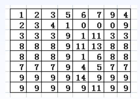
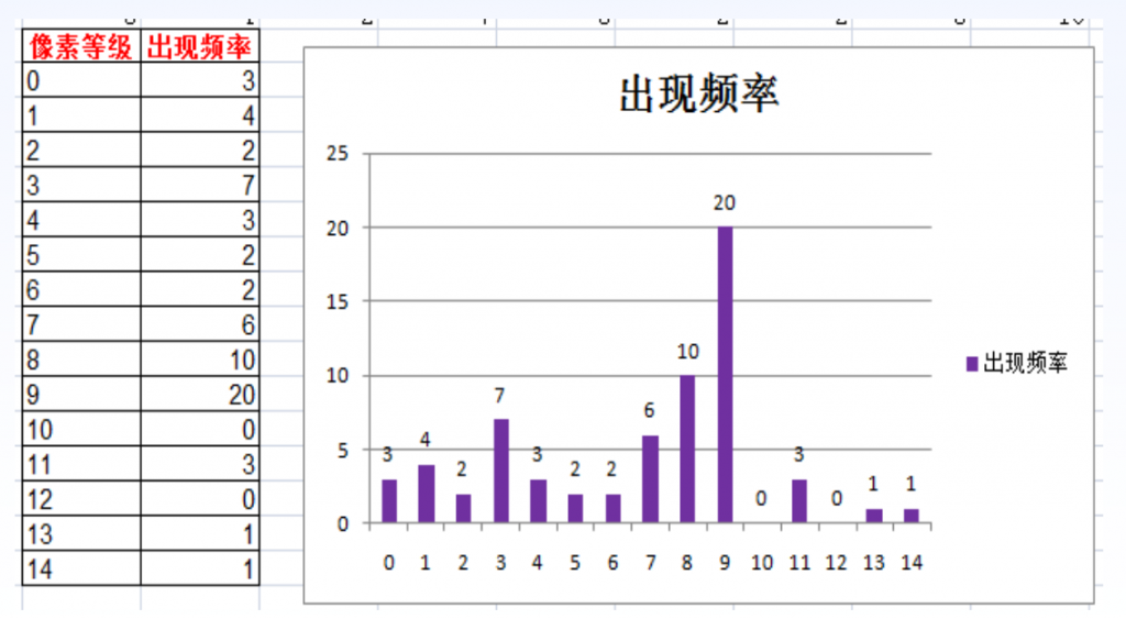
统计不同像素值出现的频率，绘制直方图。 假设有图像数据8×8，像素值范围0~14共15个灰度等级，统计得到各个等级出现次数及直方图如图所示，每个紫色的长条叫Bin

一个Bin的灰度等级也可以不为1，而是跨多个灰度等级，例如下面另一个直方图。该图尺寸为20*20，灰度范围为0-255。

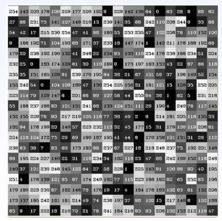
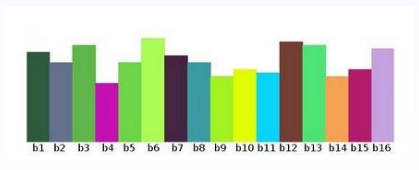
设Bin个数为16，则每个Bin包含的灰度范围有256/16=16，绘制直方图如下：

calcHist：计算图像的直方图

void calcHist( const Mat* images, int nimages, const int* channels, InputArray mask, OutputArray hist, int dims, const int* histSize, const float** ranges, bool uniform = true, bool accumulate = false );

• images：输入图像集合，可以有多张
• nimages：输入多少张图像
• channels：需要统计直方图的第几通道
• mask：只有mask中的才参与计算直方图
• hist：输出的直方图
• dims：需要统计直方图通道的个数
• histSize：直方图分成多少个区间，就是 bin的个数
• ranges：统计像素值的区间
• uniform：是否对得到的直方图数组进行归一化处理
• accumulate：在多个图像时，是否累计计算像素值得个数

normalize：归一化。在绘制直方图的时候可以使用，为了防止有的像素值出现频率比较大，有的很小，最大最小值差异可能比较大，绘制出来的直方图不好看。

void normalize( InputArray src, InputOutputArray dst, double alpha = 1, double beta = 0, int norm_type = NORM_L2, int dtype = -1, InputArray mask = noArray());

• src：输入图像
• dst：输出图像，与输入有相同的尺寸
• alpha：归一化范围左区间
• beta：归一化范围右区间
• norm_type：归一化方式
  • NORM_INF
  • NORM_L1
  • NORM_L2
  • NORM_MINMAX
• dtype：用于控制输出的图像类型。当为负数时，输出与输入有相同的类型，否则，只具有相同数量的通道，深度为CV_MAT_DEPTH(dtype)
• mask：掩模

    // Norm to probability (total count)
    // sum(numbers) = 2.0 + 8.0 + 10.0 = 20.0
    // 2.0      0.1     (2.0 / 20.0)
    // 8.0      0.4     (8.0 / 20.0)
    // 10.0     0.5     (10.0 / 20.0)
    normalize(positiveData, normalizedData_l1, 1.0, 0.0, NORM_L1);

    // Norm to unit vector: ||positiveData|| = 1.0
    // 2.0      0.15     (2.0 / sqrt(4.0 + 64.0 + 100.0))
    // 8.0      0.62     (8.0 / sqrt(4.0 + 64.0 + 100.0))
    // 10.0     0.77     (10.0 / sqrt(4.0 + 64.0 + 100.0))
    normalize(positiveData, normalizedData_l2, 1.0, 0.0, NORM_L2);

    // Norm to max element
    // 2.0      0.2     (2.0 / 10.0)
    // 8.0      0.8     (8.0 / 10.0)
    // 10.0     1.0     (10.0 / 10.0)
    normalize(positiveData, normalizedData_inf, 1.0, 0.0, NORM_INF);

    // Norm to range [0.0;1.0]
    // 2.0      0.0     (shift to left border)
    // 8.0      0.75    (8.0 - 2.0) / (10.0 - 2.0) = (6.0 / 8.0)
    // 10.0     1.0     (shift to right border)
    normalize(positiveData, normalizedData_minmax, 1.0, 0.0, NORM_MINMAX);